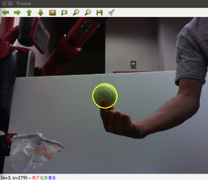
Ball Detection
Our project intended to catching the ball at 3d dimension at first.
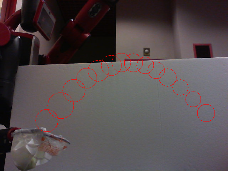
However, due to the low frequency of our 2D camera (25Hz), we cannot read the radius of tennis ball and then get the distance accurately, so we decided to make the ball fly on a 2D plane. You can see the circle is big or small. Actually, the position is also not that accurate, but it is enough for us to predict the trajectory.
Also, we can easily extend it into 3D space by add one more camera or just use a camera with faster shutter speed.
- In physical model, we use the first 3 points as well as their time intervals for prediction.
- In machine learning model, we choose the first 5 points as a set of training data.
|
|
Physical Model
Physical model is a more practical model as we can apply it to any system and any condition.
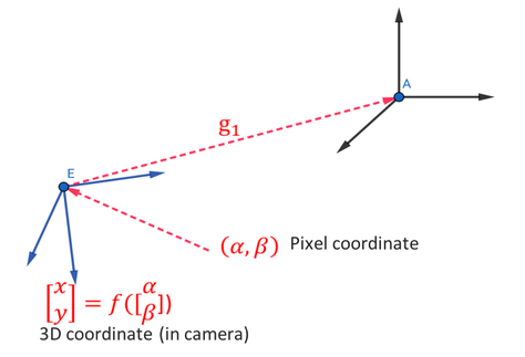
Firstly, we change the position of pixel unit into meter unit. To do this, we manually put the ball at several positions with constant distance in pixels and measure the corresponding distances in meter in camera frame by hand. Then, the relationship between pixel representation and meter representation matches.
Secondly, we use AR tags to determine the transformation from camera frame to robot base frame. We attach an AR tag on the camera and use \emph{tf} package. After finding the transformation matrix, we store it for further calculation.
- Step I: System calibration:
Firstly, we change the position of pixel unit into meter unit. To do this, we manually put the ball at several positions with constant distance in pixels and measure the corresponding distances in meter in camera frame by hand. Then, the relationship between pixel representation and meter representation matches.
Secondly, we use AR tags to determine the transformation from camera frame to robot base frame. We attach an AR tag on the camera and use \emph{tf} package. After finding the transformation matrix, we store it for further calculation.
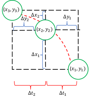
- Step II: Calculate physical parameters: After we obtain the pixel coordinates of first three data points and the time intervals of tennis ball, firstly we transform it into Cartesian coordinate of camera, then we fit the trajectory of the ball by a parabola model. We define the following pipeline to find the prediction point:
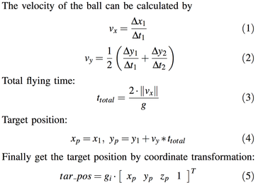
- Step III: Rules of prediction: Because we need enough time for robot arm to move ti desired configuration, the flying time of ball need to be maximized. So we choose the symmetric point of the first point the camera detected as the catching position.
- Step IV: inverse kinematics: With the help of ROS package pykdl, we can calculate the inverse kinematics of predicted position and send that to controller.
Physical model
|
Inverse kinematics
|
Machine Learning Model
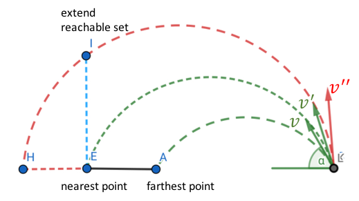
Step 1: Determine the reachable set of the Baxter arm.
In a two dimensional space, the trajectory of a flying ball is a parabola. we can always use a 1 dimensional hyper-plane to intersect those concave parabolas at a certain level. Finally, we define the reachable set of the Baxter arm to be two orthogonal 1 dimensional hyper planes.
In a two dimensional space, the trajectory of a flying ball is a parabola. we can always use a 1 dimensional hyper-plane to intersect those concave parabolas at a certain level. Finally, we define the reachable set of the Baxter arm to be two orthogonal 1 dimensional hyper planes.
Determine the Reachable Set
Step 2: Grid the reachable set & Collect data
To guarantee the training data occupies the whole reachable set, we can mesh the reachable set by a certain step size.
While collecting the data,
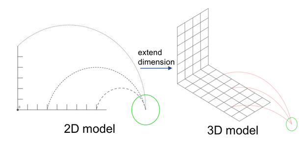
This procedure is easy to be generalized to a 3D space. Only by adding one axis and meshing the two hyper-planes in the same way as described above, we can extend the method to a 3D case.
To guarantee the training data occupies the whole reachable set, we can mesh the reachable set by a certain step size.
While collecting the data,
- Move the end effector of the Baxter arm to a node on the grid.
- Record the position of the node in the Baxter base frame as the label.
- Record the coordinates of first five points of the ball along the parabola trajectory and stack them up as a row of the feature matrix.
- Repeat the procedure above until the end effector moves through all nodes on the grid.
This procedure is easy to be generalized to a 3D space. Only by adding one axis and meshing the two hyper-planes in the same way as described above, we can extend the method to a 3D case.
Grid the Reachable Set
Step 3: Train the data
Since the training data are collected by meshing the whole space, they evenly disperse the reachable set of the Baxter arm. In this case, K-NN will be a good choice for us to try. The value of k is determined by exhaustive search. Here we choose k=5.
We have collected 284 training data in total. After applying K-NN algorithm,
As long as the error is smaller than the radius of the tennis ball, which is between 6.541 centimeters to 6.858 centimeters, the Baxter arm can catch the ball. Therefore, 1.6 cm validation error reaches the minimum requirement. It can also be inferred from the values of two errors that this is still an underfitting model. Its performance can still be improved by collecting more data.
Since the training data are collected by meshing the whole space, they evenly disperse the reachable set of the Baxter arm. In this case, K-NN will be a good choice for us to try. The value of k is determined by exhaustive search. Here we choose k=5.
We have collected 284 training data in total. After applying K-NN algorithm,
- The training error is 0.02 (2 cm).
- The validation error is 0.016 (1.6 cm).
As long as the error is smaller than the radius of the tennis ball, which is between 6.541 centimeters to 6.858 centimeters, the Baxter arm can catch the ball. Therefore, 1.6 cm validation error reaches the minimum requirement. It can also be inferred from the values of two errors that this is still an underfitting model. Its performance can still be improved by collecting more data.
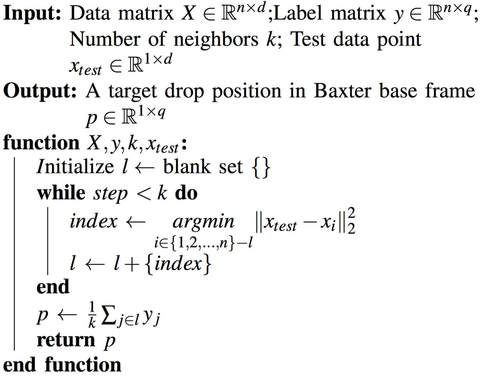
Algorithm Flow of K-NN
